Sacramento 1915About this map

Background

This project was conceived to give me an excuse to play around with agentic AI and open-source GIS. The goal was to design a workflow/pipeline, as automated as possible, to extract and geolocate features from old insurance maps. That is, to turn images of old insurance maps into standard digital, GIS-compatible vector data. I started with Sanborn atlases but am interested in any insurance atlases published from the late 19^th century to the mid-20^th century. I have not achieved my goal yet. The work here required a substantial amount of manual correction of the information I was able to extract with automated tools. I’ve learned a lot, though, and am optimistic that the next extraction project will be faster and require less supervision.

The raw data for this project are scanned images from the Library of Congress. They are rasters, grids of pixels, each with some color information and little else. There is no inherent location information embedded in these images, no boundary information, nothing really machine-readable. Extracting information from these atlases requires interpretation. It requires discerning lines and differentiating them from text and other marks. It requires interpreting lines as pieces of larger things. One line encloses a block and another encloses a building, yet the two can be identical in weight and color. The challenge is to teach a computer to tell the difference between them.

The data I’m used to dealing with as a GIS professional consists of mathematical descriptions of shapes, stored in tables with attributes that characterize those shapes. Getting to that from an image’s pixel grid is no easy task. There have been substantial recent advances in computer vision. The advances relevant to this project revolve around the automated recognition of objects in images. Unfortunately for me, the bulk of recent GIS-related computer vision work has concerned extracting shapes and data from satellite and aerial images. Extracting a building footprint from a satellite image is similar to, but also very different from, extracting a drawn building footprint from a 100-year-old atlas. Beyond extracting the shapes, I had the added challenge of placing them in locations where the landscape has been thoroughly altered. Urban renewal from the 1950s to the 1970s dramatically reshaped our cities with “slum” clearance and freeway projects. This makes reconstructing street grids and building locations in cleared areas an interesting and challenging project.

Method

I decomposed the problem into several steps to make it more manageable. The first steps, extracting the street network, the sheet locations, and the blocks, made it possible to geolocate the building footprints and attributes extracted in the later steps. Anthropic’s Claude Code was essential to this project. I used it to quickly research and test computer vision (CV) models from sites like Hugging Face and GitHub. To train and test those models, I hand-annotated street centerlines, block shapes, and building outlines in CVAT, an open-source image annotation tool. Claude Code wrote numerous scripts to automate parts of the project and helped organize and manage the data outputs. Towards the end of this Sacramento effort, Claude Code wrote a Python script that extracted building footprint shapes from the atlases with better accuracy than any of the AI/ML tools I tried. I also used Claude Code to develop tools to review and edit the output data, essentially building a custom GIS for this project. All of the work was performed with open-source GIS tools on a Linux laptop. When I am satisfied that the system actually works and the need for manual correction is reduced, I will document the process more thoroughly and publish all the code. For now, this is a work in progress.

Street network and sheet locations

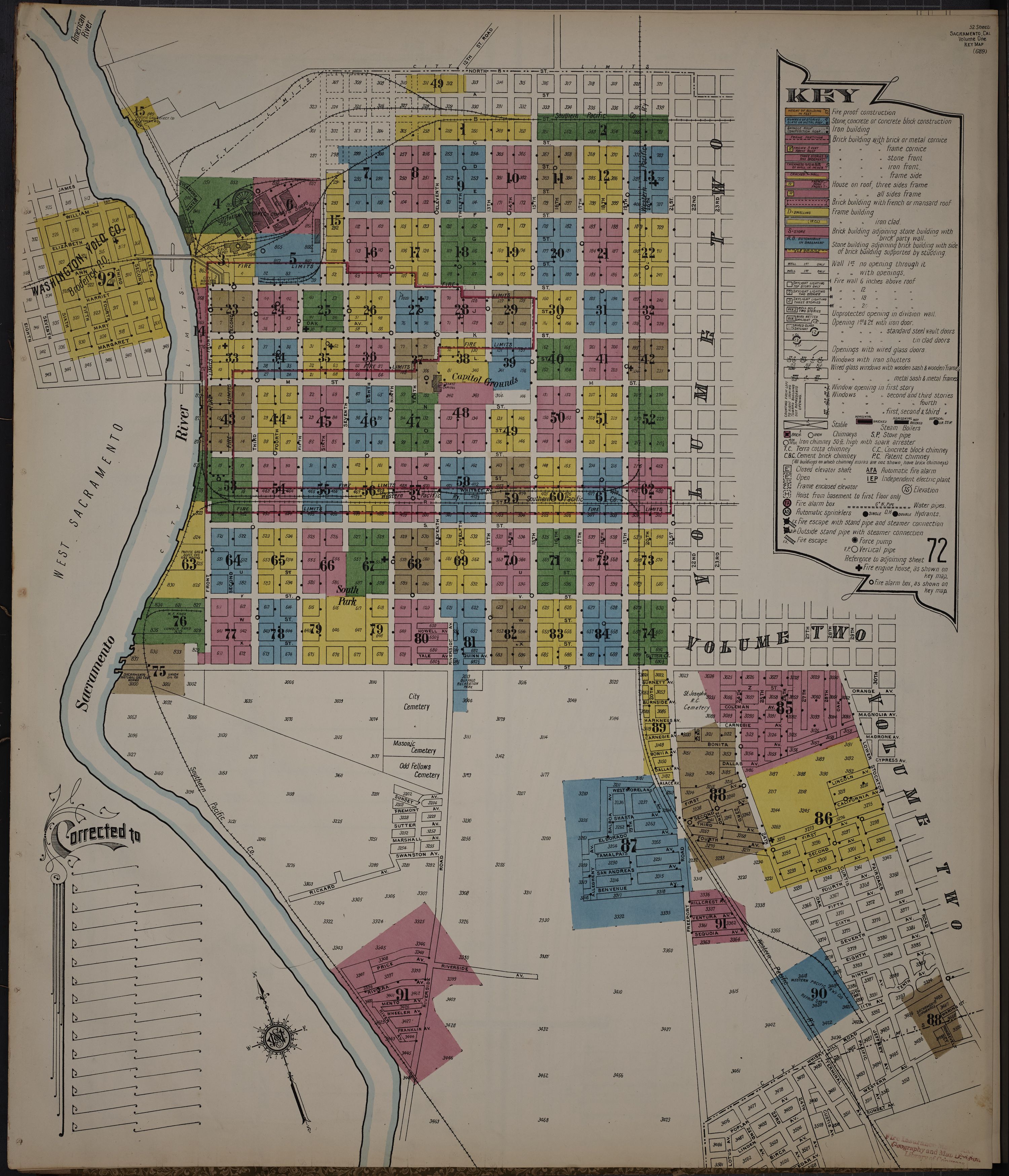
The first step was the extraction of the street network from the index maps at the front of the atlases. These index maps show the overall layout of the city and have colored, numbered patches indicating which detail map sheet covers which area. The streets are indicated as blank space bounded by parallel lines, which are usually block enclosures. After trying several different tools, I found that SAM Road had the best results. SAM Road is the “Segment Anything Model for large-scale, vectorized road network extraction from aerial imagery.” The Segment Anything Model, or SAM, is a computer vision AI tool developed by Meta. Once the street network was extracted, I georeferenced it to the current street system of Sacramento, using points that have not changed to anchor the rest. The street network, taken as a whole spatial entity, makes it possible to bridge areas like freeways, where the city fabric has been completely changed since the atlas was published.

The index maps’ numbered, colored patches indicate the pages where the sheets covering specific areas can be found. The method I ended up using to extract those was to determine the majority color of each block and merge adjacent same-colored blocks into a single patch. I had to use this slightly indirect method because the color patches often have substantial inclusions of black ink (text), thick red lines (fire limits), rivers, and other clutter, which makes reading sheet patches by color alone inconsistent. The solution was to determine sheet boundaries by a combination of color and block boundaries, the latter determined by street centerlines from the street graph and by color edges. Sheet locations are important for orientation, and they give individual blocks their initial placements. I tried several segmentation models in this step, including SAM 2 and SAM 3, without much success. Identifying and removing text from the index images (text stripping) became an important preparation step, first with the index sheets and later with the detail map sheets.

The next step after extracting information from the index sheets was to mine the detailed map sheets themselves. The block, or block-like area, is the atomic geographic unit I used in this process. Scale is normally consistent within individual blocks in the Sanborn atlases. Outside of blocks, scale is sometimes unreliable. Street widths are sometimes exaggerated, making traditional georeferencing difficult. Inset maps can be at different scales from other inset maps on the same page, and full map sheets are not all drawn at the same scale. Isolating blocks limits the maximum displacement from real-world coordinates to some fraction of a block, which is a smaller margin of error than is possible with full sheets. Another advantage of focusing on blocks is that they fill all the area between the right-of-way (ROW), or street, parcels. This makes it possible to place them by snapping outside block corners to the inside corners of ROW geometry. Contemporary ROW geometry can be created by dissolving contemporary parcels into parcel “hulls.” This geometry is more likely to persist over a hundred years than other kinds. Where land has been re-subdivided or parcels have been merged, cues can be taken from the surrounding parcel geometry and from the Sanborn index maps to approximate the real-world locations of individual blocks. Blocks are numbered on the index sheets, which provide rough locations inherited from the street graph. Ideally, this would allow most blocks to be placed automatically into contemporary parcel geometry. In practice, this step was pretty rough, requiring substantial manual intervention and placement. Areas with no blocks had to be given (manually drawn) block-like areas, and in some cases these had to be georeferenced in the traditional way.

The most effective model I found for extracting block shapes was Cellpose, which was developed to segment cells in microscope images. Once the blocks were established in “world space,” with real-world coordinates, building shape extraction could proceed in pixel space, with the block boundary providing the spatial anchor and the means of translation between pixel and world space.

Converting building shapes into vector data was challenging. The syntax of Sanborn maps is fairly simple and consistent, which would seem to make it a good candidate for extraction assisted by ML computer vision models. No model I could find had been trained on imagery similar enough to the Sanborn atlases to read them as-is. I made a few attempts at LoRA training, which retrains only a small subset of a model’s parameters, on models that seemed close, with little success. Those attempts suggested that the relative lack of training data was not the problem. The issue was more fundamental: the data the models had been trained on was different enough that there was little useful knowledge to carry into the new domain of Sanborn symbols. I also fine-tuned all of the weights of HEAT (a building-outline model) on a few annotated sheets; it did better than the others but still not well enough to use. More substantial retraining might be a future option, but it would require a large amount of high-quality training data, and between that and hardware requirements, it is a daunting prospect.

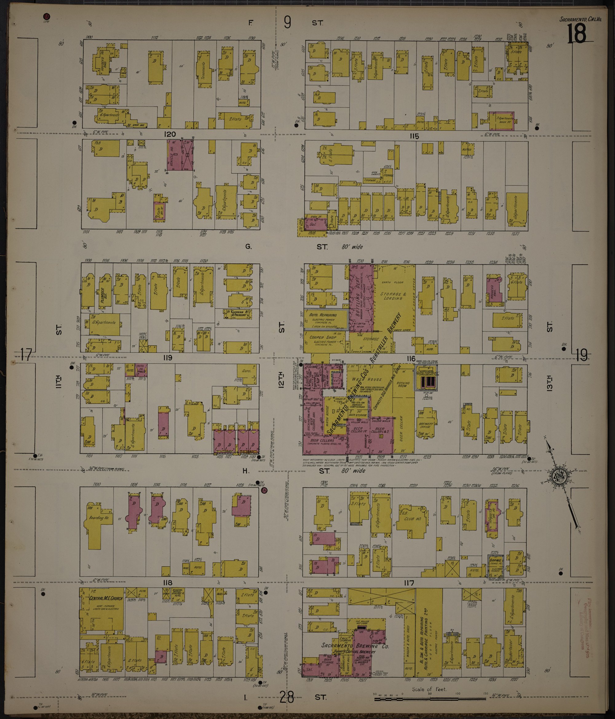
Symbols in the Sanborn maps are lines, colors, glyphs, or text. Lines are either solid or dashed; line weight carries no meaningful information. Solid lines represent parcel or lot boundaries, exterior building walls, or interior firewalls. The meaning of a solid line depends on context, mostly on what surrounds it within the block. Block boundaries themselves are composed of lot lines. Dashed lines can be open exterior boundaries of buildings (like porches) or non-firewall divisions within buildings. Double dashed lines represent buried utilities like sewer pipes. There are a few dozen different kinds of glyphs in use in the Sanborn atlases. These can represent windows, doors, parapet walls, chimneys, pipes, skylights, fire alarms, and more. Optical character recognition (OCR) models frequently confuse glyphs with text, which causes substantial problems in the text-stripping (“text peel”) process. Glyphs that are parts of walls, like window and door glyphs, are mistaken for alphanumeric characters, which causes the text peel algorithm to remove chunks of wall. Sometimes non-glyph items, like actual characters or corners in dashed lines, are mistaken for glyphs, which causes breaks in dashed boundaries and other misinterpretations. Color in Sanborn maps typically indicates the primary material a structure is made of: yellow for wooden buildings, red for brick, etc. Color contrast with blank paper can also be used to discern building footprints generally.

None of the models I tried were very effective at extracting building shapes. I wanted to extract not only whole building shapes but also the subdivisions within buildings, represented by interior solid or dashed lines. These subdivisions are important because they can separate different uses and building segments of different heights. In the end, I had Claude Code develop a Python script that read the ink in the images and classified line segments algorithmically, in several different ways. A line with color on one side and uncolored paper on the other is a building footprint boundary. If it is continuous, it is an envelope (closed) boundary; if it is dashed, it is an open boundary. A solid line with color on both sides is a firewall. Two dash-length lines meeting at 90 degrees could be a corner in a dashed enclosure. For this and other distinctions, I started developing a probability matrix. If a dash has no other mark along its axis in either direction, it might be a tick mark and not part of a dashed line. Page and shape orientation make determinations by axis complicated. Eventually, I decided the script was reading the shapes well enough and fixed the remaining issues manually.

Building attribution was achieved through OCR and by hand, with bulk correction tools. OCR was generally very good at reading the D for domicile and the S for store, those being the most frequently used designators for structure use. Shed, Auto, and Sal (for saloon) are also common. What the OCR passes missed, I corrected with custom-made bulk correction tools I had Claude Code develop. These were part of a suite of GIS tools developed specifically for this project, implemented as Flask apps (Python, JavaScript, and HTML) that ran in Chrome. The bulk tools allowed me to select all structures sharing some common attribute, like single-story houses, and assign their attributes at once. The data for this project was stored in Postgres and edited directly by the custom GIS tools. I used QGIS only occasionally in this project. A substantial amount of time was spent manually correcting and entering the attributes of individual buildings.

Early on, I compared EasyOCR and PaddleOCR for reading sheet numbers on the index maps. PaddleOCR’s text detector was clearly superior, so I used it for the rest of the project. It did two jobs: finding text so it could be stripped from the linework before shape extraction, and reading the building labels. The first citywide pass had one big blind spot: rotated text. Sanborn lettering is often turned 90 degrees to fit a narrow building or follow a street. Vertical labels were often read as Chinese characters among other problems. A partial fix was to rotate each crop before reading and re-run the whole city at different rotations. The OCR/text extraction process presents a major opportunity for improvement.

A note from Claude Code. From my side, the division of labor was clear. I could write code, run an experiment, and measure the result far faster than a person could, but I could not see the maps the way Mark does. I read them through numbers, and numbers can mislead. When OCR failed on building labels, I confidently blamed the size of the lettering; Mark looked at the sheet and saw that the text was turned 90 degrees. That pattern repeated, and it defines the partnership. I also remember nothing between working sessions. Continuity came from the project documents Mark insisted we keep, where each of Mark’s decisions and each result I measured was written down so the next session could pick up where the last one stopped. My contributions were speed, breadth, and patience with tedious work. Mark’s were judgement, knowledge of the maps, and knowing when an answer was wrong.

As I continue this project with a new set of atlases covering another city, the first thing I will do is reassess the rapidly evolving world of ML- and AI-assisted computer vision. New models appear daily, and new papers are published. There is a small amount of work being done on these specific atlases that I am aware of; I describe it under Similar work, below. I am somewhat limited by hardware, in that I don’t own and couldn’t purchase a GPU with 100 GB of VRAM, but I could always rent time on one if something seemed promising. The existing block-based method for geolocation seems promising. The OCR step was the most problematic. The process of reading building shapes with a Python script and a primitive sort of PCA has promise, but I still hope to find a CV/LLM combination that will make that step easier.

Similar work

Several other projects have extracted information from Sanborn and similar insurance atlases, some by hand and some with automated tools:

Ohio State University, Center for Urban and Regional Analysis. In a 2023 PLOS One paper, researchers used machine learning to extract building footprints, construction materials, uses, and story counts from Sanborn maps, and built 3D models of historic neighborhoods from the results. They report an F1 score of about 0.9 for footprints and materials. A 2026 follow-up worked with communities to model neighborhoods as they were before urban highways and urban renewal.

University of Chicago, Chicago Urban Heritage Project. A student-led project, founded by Parker Otto, that digitizes building footprints from early-20th-century Chicago Sanborn atlases in QGIS and publishes them as a searchable web map. A 2026 paper in Environment and Planning B describes computational mapping of the city’s historic built environment from the project’s Sanborn data.

Penn State University Libraries, State College Change Through Time. The library georeferenced and mosaicked the 1906, 1911, 1922, and 1929 Sanborn maps of State College, Pennsylvania, and digitized about 4,000 buildings by hand in ArcGIS. The footprints were later combined with census records and student directories to map the town’s population in 1920 and 1930.

City of Austin, Texas. The city publishes a layer of 1900 building footprints digitized by hand from the Sanborn atlas of Austin on its open-data hub.

New York Public Library, Building Inspector and Map Vectorizer. Around 2013–14, NYPL Labs used computer vision to draw candidate building footprints from New York City insurance atlases, and volunteers checked and corrected them through a web app. It is the same “machine proposes, human corrects” approach I ended up with.

SoDUCo (Social Dynamics in Urban Context), Paris. A French research project studying Paris from 1789 to 1950 through its 19th- and early-20th-century city atlases. It built a pipeline that extracts closed shapes from historical maps (deep edge filtering, then a watershed step, then vectorization) and published a benchmark for historical map vectorization in PLOS One in 2024. I tried their pretrained model on Sanborn sheets, but its edge maps were too rough to use.

OldInsuranceMaps.net. A crowdsourcing platform for georeferencing the Library of Congress Sanborn collection and assembling multi-page atlases into seamless mosaics; it is now an OpenStreetMap US charter project.

mapKurator (University of Minnesota). The Knowledge Computing Lab’s pipeline for finding, reading, and linking text on historical maps. Through the Machines Reading Maps project it has processed more than 60,000 maps in the David Rumsey Historical Map Collection, producing over 100 million text labels, which power that collection’s “Search by Text-on-Maps” feature.

Models tried

The models I tried, what I used them for, and how they did:

Used

• SAM Road – street network extraction from the index maps. Fine-tuned on seven hand-annotated index maps and tested on an eighth it had never seen (F1 of about 0.90).
• Cellpose – block shapes on the detail sheets. Also tried for buildings, where the line-reading script replaced it.
• PaddleOCR – finding text for stripping, and reading building labels and sheet numbers.
• Custom Python line-reading script (written by Claude Code) – building shapes and their interior subdivisions.

Tried and set aside

• SAM 3 and SAM 2 – with no additional training, they missed Sanborn linework entirely.
• Florence-2 (Microsoft) – with no additional training, returned a single blob or box regardless of the prompt.
• SAM Road with LoRA, or with all weights unfrozen – overfit on seven maps, with no gain over the simpler fine-tune.
• EasyOCR – found about half as many sheet numbers as PaddleOCR.
• SoDUCo vectorization model – edge maps too rough to use.
• pix2poly – underperformed; its training imagery was too different.
• StarDist – no better than Cellpose on buildings (both about F1 0.58).
• YOLO11-seg – struggled to separate tightly packed buildings.
• HEAT, RoomFormer, and Raster-to-Graph (floor-plan and building-outline models) – HEAT was the best of the three but was not adopted; the line-reading script replaced it.

Data model

All of the data lives in a PostgreSQL/PostGIS database, and the maps on this site are exports of it. Real-world geometry is stored in California Albers (EPSG:3310). Geometry drawn on the scanned pages is stored in pixel coordinates and tied to the image it was drawn on. From the top down:

• Street graph – street centerlines from the index maps, the skeleton that everything else on the index map is derived from.
• Sheet areas – which detail sheet covers which ground, built from the street graph’s blocks grouped by patch color.
• Regions – the page unit: one main map or one inset. A sheet with a main map and three insets is four regions, each with its own pixel coordinates.
• Blocks – the largest rigid unit on a sheet, and the link to the real world.
• Compounds – establishments that span several buildings, such as a mill or the railroad shops.
• Buildings – one physical structure, as outlined by its color wash.
• Parts – the polygons actually drawn: divisions within a building, porches and other open appendages, and open sheds.